Predictive Analysis
Predict whether an event is attractive
Classification & Hypothesis Testing
Prediction with 19 Variables
We implemented 5 classification methods to predict if an event is popular. We used all the variables as predictors, excluding number of participants and the response variable “attractive_events”, because the response variable is categorized based on the number of participants. To evaluate the performance of these models, we split the dataset into 80% of training data and 20% of test data and calculated accuracy of the trained model on test data. At the first glance, the accuracy for these models are better than random guess, which is ideal. However, if we take a further look at the confusion matrix of each model, we find the precision of predicting unattractive events is pretty low relative to precision of predicting attractive events. This means there are way more unattractive events than attractive events in our dataset. Among the 5 classifiers, SVM returned relatively high precision for both categories. With that being said, we determine that SVM performed the best.
KNN: 0.709202 (0.022229)
DT: 0.707975 (0.024639)
RF: 0.727607 (0.027311)
NB: 0.727198 (0.020393)
SVM: 0.731084 (0.019080)
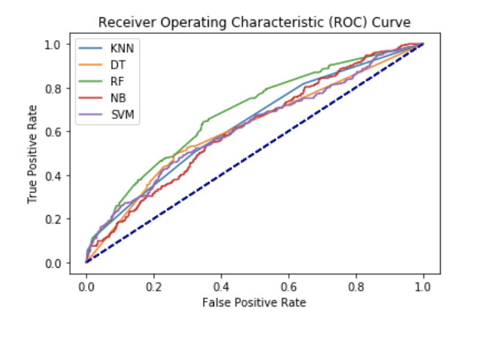
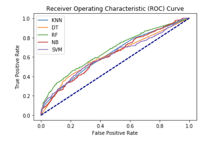
We performed cross-validation, which repeats the train-validate split inside the training data. Here is the mean accuracy and standard deviation of it for the five methods. As we mentioned, we cannot simply choose the optimal model based on the accuracy, because with extreme cutoffs or highly unbalanced data set, the accuracy may be high, but it will not be the same case for true positive rate or false positive rate. In order to select best prediction model, we plot ROC curve. Normally we use 0.5 as the probability assigned to each observation, but sensitivity(tpr) decreases as the cutoff is increased, while specificity(fpr) increases as the cutoff increases. Therefore, Instead of manually checking probability cutoffs, we created an ROC curve which will sweep through all possible cutoffs, and plot the sensitivity (true positive rate) against the false positive rate (specificity). We observe the area under Random Forest is the largest, and the area under Decision Tree is the smallest. We determine Random Forest to be the best classfier.
Feature Selection
Univariate Selection
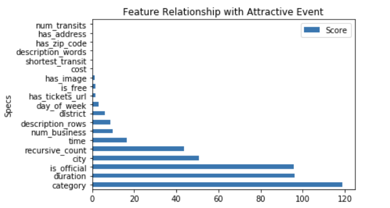 Statistical tests can be used to select those features that have the strongest relationship with the output variable.
The scikit-learn library provides the SelectKBest class that can be used with a suite of different statistical tests to select a specific number of features.
The example below uses the chi-squared (chi²) statistical test for non-negative features to select 19 of the best features from the Dataset.
Prediction with 13 Variables
KNN: 0.711656 (0.018854)
DT: 0.701022 (0.023133)
RF: 0.722495 (0.027346)
NB: 0.727198 (0.020474)
SVM: 0.734151 (0.016283)
Selected features:
'has_image',
'is_free',
'has_tickets_url',
'day_of_week',
'district',
'description_rows',
'num_business',
'time',
'recursive_count',
'city',
'is_official',
'duration',
'category'
Prediction with 10 Variables
KNN: 0.709202 (0.022229)
DT: 0.707975 (0.024639)
RF: 0.727607 (0.027311)
NB: 0.727198 (0.020393)
SVM: 0.731084 (0.019080)
Selected features:
'day_of_week',
'district',
'description_rows',
'num_business',
'time',
'recursive_count',
'city',
'is_official',
'duration',
'category'
Prediction with 5 Variables
KNN: 0.716360 (0.023443)
DT: 0.749489 (0.023375)
RF: 0.746830 (0.023060)
NB: 0.727812 (0.020480)
SVM: 0.740695 (0.020425)
Selected features:
'recursive_count',
'city',
'is_official',
'duration',
'category'
Hypothesis I
-
-
Interpretation: For one-unit increase in num_business, recursive_counts will be increased by 0.0059
H0: All the factors are statistically significant for predicting how many times an event is repeated
HA: At least one factor does not have a relationship with how many times an event is repeated
We conclude the following independent variables are statistically significant:
description_words: count of words in an event description
duration: duration of an event
day_of_week: 0-6 represents Monday-Sunday correspondingly
shortest_transit: the distance from an event to the closest transportation
num_business: number of businesses around an event within 1 km
From the summary plot, we found the equation for our linear regression model to be:
recusive_count = 64.3301 - 2.2243*description_words- 0.3132*duration
+ 1.0808*day_of_week -0.0261*shortest_transit +0.0059*num_business
Hypothesis II
-
-
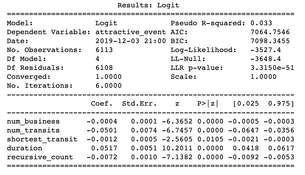
Interpretation: The coefficient for duration= 0.0517 which is interpreted as the expected change in log odds for a one-unit increase in the duration.
The odds ratio can be calculated by exponentiating this value to get 1.053 which means we expect to see about 5.3% increase in the odds of being an attractive event, for a one-unit increase in duration.
H0: All the factors are statistically insignificant for predicting the probability of an attractive event
HA: there is significant relationship between the attractive events and at least one of the independent variables
We conclude the following independent variables are statistically significant:
num_transits: number of transportations within 500m of an event
duration: duration of an event
recursive_count: how many times an event is repeated
shortest_transit: the distance from an event to the closest transportation
num_business: number of businesses around an event within 1 km
From the summary plot, we found the equation for our logistic regression model to be:
P(attractive_evets) = -0.0004*num_business-0.0501*num_transits +0.0517*duration
-0.0072*recursive_count -0.0012*shortest_transit
Hypothesis III (part1)
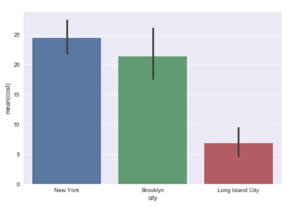
H0: the mean attendance for events held in New York, Brooklyn, and Long Island City are the same.
HA: the mean attendance for events held in New York, Brooklyn, and Long Island City are not the same.
Hypothesis III (part2)
H0: the mean attendance for events held in New York, Brooklyn, and Long Island City are the same.
HA: the mean attendance for events held in New York, Brooklyn, and Long Island City are not the same.
Conclusion
Based on the above analysis, recursive_count, city, is_official, duration, category these five factors could achieve the highest prediction accuracy. Albeit from the hypothesis testing II, the selected statistically significant features are num_business, num_transits, shortest_transit, duration and recursive_count, after dropping the statistically insignificant features. Interestingly, we also notice that recursive_count has negative association with the possibility of an event being popular, which might suggest that the repeated events are held due to organizational routine, instead of popularity. It is supported by hypothesis testing I that these repeated events tend to have shorter description and duration, and to be held near business circle but not necessarily to be transportation-wise convinient to attend. Furthermore, comparison between the mean cost and mean participants among New York, Brooklyn and Long Island City shows that hosts can choose to hold events in Long Island City instead of New York with relatively less cost but without sacrificing number of participants. With that being said, it would be helpful for hosts to consider recursive_count, city, is_official, duration, category, num_business, num_transits, shortest_transit when holding events.
